| Fundamentals of Statistics contains material of various lectures and courses of H. Lohninger on statistics, data analysis and chemometrics......click here for more. |

|
Home  Statistical Tests Means and Medians One Sample t-Test Large Sample Size Statistical Tests Means and Medians One Sample t-Test Large Sample Size |
|
| See also: survey on statistical tests, small samples, two-sample t-test, distribution calculator |   |
One-Sample t-Test - Large Samples
Let's assume that we have to fill containers with an expensive substance. Our customers expect a guaranteed quantity μ of the material. We know the precision σ of our machinery and want to check whether we have adjusted our dispenser correctly. Since measurements are rather cheap (i.e. we only have to weigh the container) we can afford a lot of measurements n. The question we have to answer is how large does the mean quantity have to be, so that we don't have to reject the assumption that our filling procedure is correct. Since we have to acknowledge the possibility of an erroneous decision, we are content when our error probability is smaller than α%. The probability α is called the confidence level. The decision can be made according to the table below:
1. We have to formulate our two hypotheses (the null hypothesis H0 and the alternative hypothesis H1): H0: amount <= limit H1: amount > limit 3. In order to decide which of the two hypotheses is true we calculate the test statistic
which is normally distributed. The z-value gives us the distance of
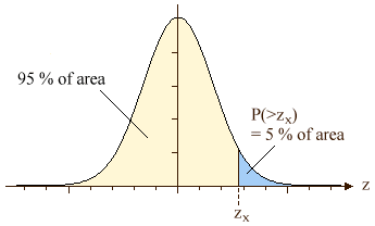
the measured 4. Defining the region of rejection. In order to know when we have to
reject the null hypothesis (i.e.
5. Finally, we have to select the appropriate hypothesis by inserting
the numerical values for Note: A more general approach is to use the t-distribution for testing,
since the t-distribution approaches the normal distribution for large sample
sizes.
|
|
| Home Statistical Tests Means and Medians One Sample t-Test Large Sample Size |
|